##
## Attaching package: 'dplyr'
## The following objects are masked from 'package:stats':
##
##     filter, lag
## The following objects are masked from 'package:base':
##
##     intersect, setdiff, setequal, union
## here() starts at /Users/zhihanxian/MADA2021/ZhihanXian-MADA-portfolio
## ── Attaching packages ─────────────────────────────────────── tidyverse 1.3.1 ──
## ✓ ggplot2 3.3.5     ✓ purrr   0.3.4
## ✓ tibble  3.1.5     ✓ stringr 1.4.0
## ✓ tidyr   1.1.4     ✓ forcats 0.5.1
## ✓ readr   2.0.2
## ── Conflicts ────────────────────────────────────────── tidyverse_conflicts() ──
## x dplyr::filter() masks stats::filter()
## x dplyr::lag()    masks stats::lag()
## Registered S3 method overwritten by 'tune':
##   method                   from
##   required_pkgs.model_spec parsnip
## ── Attaching packages ────────────────────────────────────── tidymodels 0.1.4 ──
## ✓ broom        0.7.9      ✓ rsample      0.1.0
## ✓ dials        0.0.10     ✓ tune         0.1.6
## ✓ infer        1.0.0      ✓ workflows    0.2.4
## ✓ modeldata    0.1.1      ✓ workflowsets 0.1.0
## ✓ parsnip      0.1.7      ✓ yardstick    0.0.8
## ✓ recipes      0.1.17
## ── Conflicts ───────────────────────────────────────── tidymodels_conflicts() ──
## x scales::discard() masks purrr::discard()
## x dplyr::filter()   masks stats::filter()
## x recipes::fixed()  masks stringr::fixed()
## x dplyr::lag()      masks stats::lag()
## x yardstick::spec() masks readr::spec()
## x recipes::step()   masks stats::step()
## • Dig deeper into tidy modeling with R at https://www.tmwr.org
## Loading required package: rpart
##
## Attaching package: 'rpart'
## The following object is masked from 'package:dials':
##
##     prune
##
## Attaching package: 'vip'
## The following object is masked from 'package:utils':
##
##     vi
## Loading required package: Matrix
##
## Attaching package: 'Matrix'
## The following objects are masked from 'package:tidyr':
##
##     expand, pack, unpack
## Loaded glmnet 4.1-3
## #  5-fold cross-validation repeated 5 times using stratification
## # A tibble: 25 × 3
##    splits           id      id2
##    <list>           <chr>   <chr>
##  1 <split [323/83]> Repeat1 Fold1
##  2 <split [323/83]> Repeat1 Fold2
##  3 <split [325/81]> Repeat1 Fold3
##  4 <split [326/80]> Repeat1 Fold4
##  5 <split [327/79]> Repeat1 Fold5
##  6 <split [323/83]> Repeat2 Fold1
##  7 <split [323/83]> Repeat2 Fold2
##  8 <split [325/81]> Repeat2 Fold3
##  9 <split [326/80]> Repeat2 Fold4
## 10 <split [327/79]> Repeat2 Fold5
## # … with 15 more rows
## # A tibble: 1 × 3
##   .metric .estimator .estimate
##   <chr>   <chr>          <dbl>
## 1 rmse    standard        1.22
## # A tibble: 1 × 3
##   .metric .estimator .estimate
##   <chr>   <chr>          <dbl>
## 1 rmse    standard        1.22
## Decision Tree Model Specification (regression)
##
## Main Arguments:
##   cost_complexity = tune()
##   tree_depth = tune()
##
## Computational engine: rpart
## # A tibble: 25 × 2
##    cost_complexity tree_depth
##              <dbl>      <int>
##  1    0.0000000001          1
##  2    0.0000000178          1
##  3    0.00000316            1
##  4    0.000562              1
##  5    0.1                   1
##  6    0.0000000001          4
##  7    0.0000000178          4
##  8    0.00000316            4
##  9    0.000562              4
## 10    0.1                   4
## # … with 15 more rows
## ! Fold1, Repeat1: internal: A correlation computation is required, but `estimate` is const...
## ! Fold2, Repeat1: internal: A correlation computation is required, but `estimate` is const...
## ! Fold3, Repeat1: internal: A correlation computation is required, but `estimate` is const...
## ! Fold4, Repeat1: internal: A correlation computation is required, but `estimate` is const...
## ! Fold5, Repeat1: internal: A correlation computation is required, but `estimate` is const...
## ! Fold1, Repeat2: internal: A correlation computation is required, but `estimate` is const...
## ! Fold2, Repeat2: internal: A correlation computation is required, but `estimate` is const...
## ! Fold3, Repeat2: internal: A correlation computation is required, but `estimate` is const...
## ! Fold4, Repeat2: internal: A correlation computation is required, but `estimate` is const...
## ! Fold5, Repeat2: internal: A correlation computation is required, but `estimate` is const...
## ! Fold1, Repeat3: internal: A correlation computation is required, but `estimate` is const...
## ! Fold2, Repeat3: internal: A correlation computation is required, but `estimate` is const...
## ! Fold3, Repeat3: internal: A correlation computation is required, but `estimate` is const...
## ! Fold4, Repeat3: internal: A correlation computation is required, but `estimate` is const...
## ! Fold5, Repeat3: internal: A correlation computation is required, but `estimate` is const...
## ! Fold1, Repeat4: internal: A correlation computation is required, but `estimate` is const...
## ! Fold2, Repeat4: internal: A correlation computation is required, but `estimate` is const...
## ! Fold3, Repeat4: internal: A correlation computation is required, but `estimate` is const...
## ! Fold4, Repeat4: internal: A correlation computation is required, but `estimate` is const...
## ! Fold5, Repeat4: internal: A correlation computation is required, but `estimate` is const...
## ! Fold1, Repeat5: internal: A correlation computation is required, but `estimate` is const...
## ! Fold2, Repeat5: internal: A correlation computation is required, but `estimate` is const...
## ! Fold3, Repeat5: internal: A correlation computation is required, but `estimate` is const...
## ! Fold4, Repeat5: internal: A correlation computation is required, but `estimate` is const...
## ! Fold5, Repeat5: internal: A correlation computation is required, but `estimate` is const...
## Warning: This tuning result has notes. Example notes on model fitting include:
## internal: A correlation computation is required, but `estimate` is constant and has 0 standard deviation, resulting in a divide by 0 error. `NA` will be returned.
## internal: A correlation computation is required, but `estimate` is constant and has 0 standard deviation, resulting in a divide by 0 error. `NA` will be returned.
## internal: A correlation computation is required, but `estimate` is constant and has 0 standard deviation, resulting in a divide by 0 error. `NA` will be returned.
## # Tuning results
## # 5-fold cross-validation repeated 5 times using stratification
## # A tibble: 25 × 5
##    splits           id      id2   .metrics          .notes
##    <list>           <chr>   <chr> <list>            <list>
##  1 <split [323/83]> Repeat1 Fold1 <tibble [50 × 6]> <tibble [1 × 1]>
##  2 <split [323/83]> Repeat1 Fold2 <tibble [50 × 6]> <tibble [1 × 1]>
##  3 <split [325/81]> Repeat1 Fold3 <tibble [50 × 6]> <tibble [1 × 1]>
##  4 <split [326/80]> Repeat1 Fold4 <tibble [50 × 6]> <tibble [1 × 1]>
##  5 <split [327/79]> Repeat1 Fold5 <tibble [50 × 6]> <tibble [1 × 1]>
##  6 <split [323/83]> Repeat2 Fold1 <tibble [50 × 6]> <tibble [1 × 1]>
##  7 <split [323/83]> Repeat2 Fold2 <tibble [50 × 6]> <tibble [1 × 1]>
##  8 <split [325/81]> Repeat2 Fold3 <tibble [50 × 6]> <tibble [1 × 1]>
##  9 <split [326/80]> Repeat2 Fold4 <tibble [50 × 6]> <tibble [1 × 1]>
## 10 <split [327/79]> Repeat2 Fold5 <tibble [50 × 6]> <tibble [1 × 1]>
## # … with 15 more rows
## # A tibble: 1 × 3
##   cost_complexity tree_depth .config
##             <dbl>      <int> <chr>
## 1    0.0000000001          1 Preprocessor1_Model01
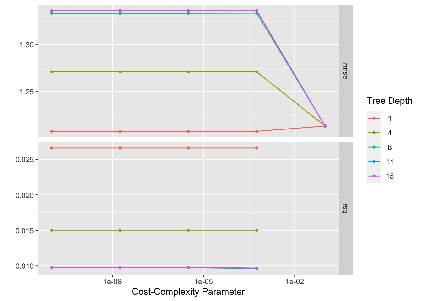
## # A tibble: 25 × 8
##    cost_complexity tree_depth .metric .estimator  mean     n std_err .config
##              <dbl>      <int> <chr>   <chr>      <dbl> <int>   <dbl> <chr>
##  1    0.0000000001          1 rmse    standard    1.21    25  0.0258 Preprocess…
##  2    0.0000000178          1 rmse    standard    1.21    25  0.0258 Preprocess…
##  3    0.00000316            1 rmse    standard    1.21    25  0.0258 Preprocess…
##  4    0.000562              1 rmse    standard    1.21    25  0.0258 Preprocess…
##  5    0.1                   1 rmse    standard    1.21    25  0.0256 Preprocess…
##  6    0.1                   4 rmse    standard    1.21    25  0.0256 Preprocess…
##  7    0.1                   8 rmse    standard    1.21    25  0.0256 Preprocess…
##  8    0.1                  11 rmse    standard    1.21    25  0.0256 Preprocess…
##  9    0.1                  15 rmse    standard    1.21    25  0.0256 Preprocess…
## 10    0.0000000001          4 rmse    standard    1.27    25  0.0256 Preprocess…
## # … with 15 more rows
# best model rmse is 1.21, std is 0.0258, the null model rmse is 1.22, std = 0. Thus, the model is not that useful.
############# LASSO model ##############
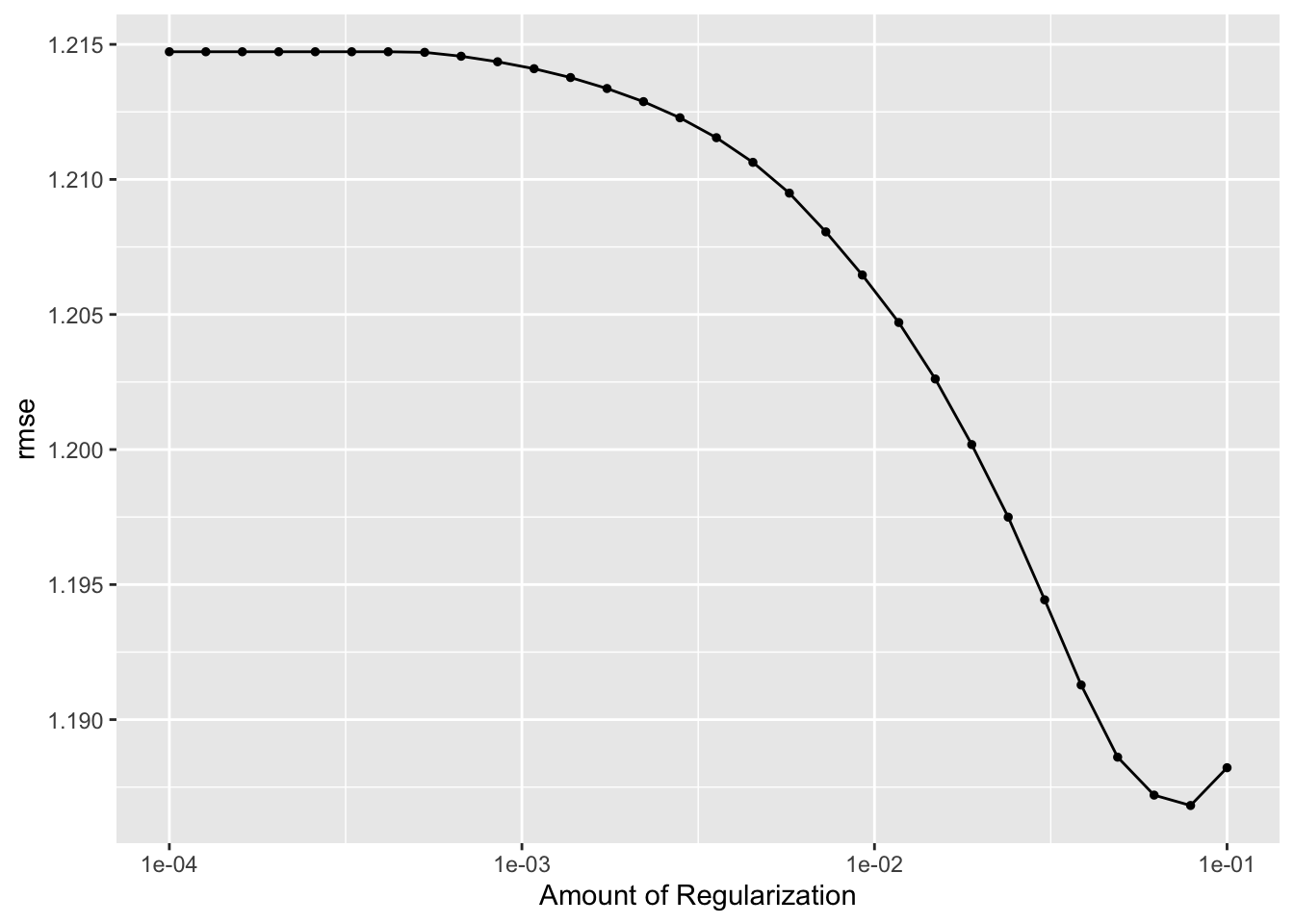
lr_mod <- linear_reg(penalty = tune(), mixture = 1) %>% set_engine("glmnet") %>% set_mode("regression")
lr_workflow <- workflow() %>% add_model(lr_mod) %>% add_recipe(data_rec)
lr_reg_grid <- tibble(penalty = 10^seq(-4, -1, length.out = 30))
lr_res <-
lr_workflow %>%
tune_grid(resamples = folds,
grid = lr_reg_grid,
control = control_grid(save_pred = TRUE),
metrics = metric_set(rmse))
b = lr_res %>% collect_metrics()
lr_res %>% autoplot()
## # A tibble: 1 × 2
##   penalty .config
##     <dbl> <chr>
## 1  0.0788 Preprocessor1_Model29

## # A tibble: 30 × 7
##    penalty .metric .estimator  mean     n std_err .config
##      <dbl> <chr>   <chr>      <dbl> <int>   <dbl> <chr>
##  1  0.0788 rmse    standard    1.19    25  0.0258 Preprocessor1_Model29
##  2  0.0621 rmse    standard    1.19    25  0.0260 Preprocessor1_Model28
##  3  0.1    rmse    standard    1.19    25  0.0256 Preprocessor1_Model30
##  4  0.0489 rmse    standard    1.19    25  0.0261 Preprocessor1_Model27
##  5  0.0386 rmse    standard    1.19    25  0.0261 Preprocessor1_Model26
##  6  0.0304 rmse    standard    1.19    25  0.0262 Preprocessor1_Model25
##  7  0.0240 rmse    standard    1.20    25  0.0263 Preprocessor1_Model24
##  8  0.0189 rmse    standard    1.20    25  0.0264 Preprocessor1_Model23
##  9  0.0149 rmse    standard    1.20    25  0.0265 Preprocessor1_Model22
## 10  0.0117 rmse    standard    1.20    25  0.0265 Preprocessor1_Model21
## # … with 20 more rows
## [1] 8
## i Creating pre-processing data to finalize unknown parameter: mtry
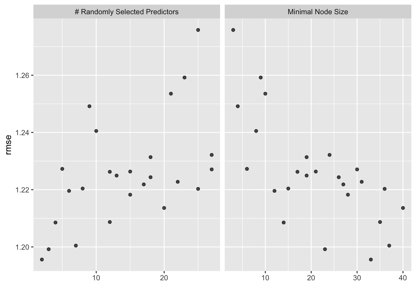
## # A tibble: 1 × 3
##    mtry min_n .config
##   <int> <int> <chr>
## 1     2    33 Preprocessor1_Model10
## # A tibble: 25 × 8
##     mtry min_n .metric .estimator  mean     n std_err .config
##    <int> <int> <chr>   <chr>      <dbl> <int>   <dbl> <chr>
##  1     2    33 rmse    standard    1.20    25  0.0258 Preprocessor1_Model10
##  2     3    23 rmse    standard    1.20    25  0.0258 Preprocessor1_Model13
##  3     7    37 rmse    standard    1.20    25  0.0259 Preprocessor1_Model25
##  4     4    14 rmse    standard    1.21    25  0.0256 Preprocessor1_Model06
##  5    12    35 rmse    standard    1.21    25  0.0257 Preprocessor1_Model15
##  6    20    40 rmse    standard    1.21    25  0.0253 Preprocessor1_Model23
##  7    15    28 rmse    standard    1.22    25  0.0253 Preprocessor1_Model03
##  8     6    12 rmse    standard    1.22    25  0.0253 Preprocessor1_Model18
##  9    25    36 rmse    standard    1.22    25  0.0249 Preprocessor1_Model09
## 10     8    15 rmse    standard    1.22    25  0.0254 Preprocessor1_Model21
## # … with 15 more rows
# best model rmse is 1.20, std is 0.0258, the null model rmse is 1.22, std = 0. Thus, the model seems to perform the same as the two models above.
############### Model Selection #################
# It looks like the 3 models have the similar rmse values, and also same std. I do not know which model tends to overfit more, I will randomly pick one.
################ Final Fit ################
# I picked random forest model
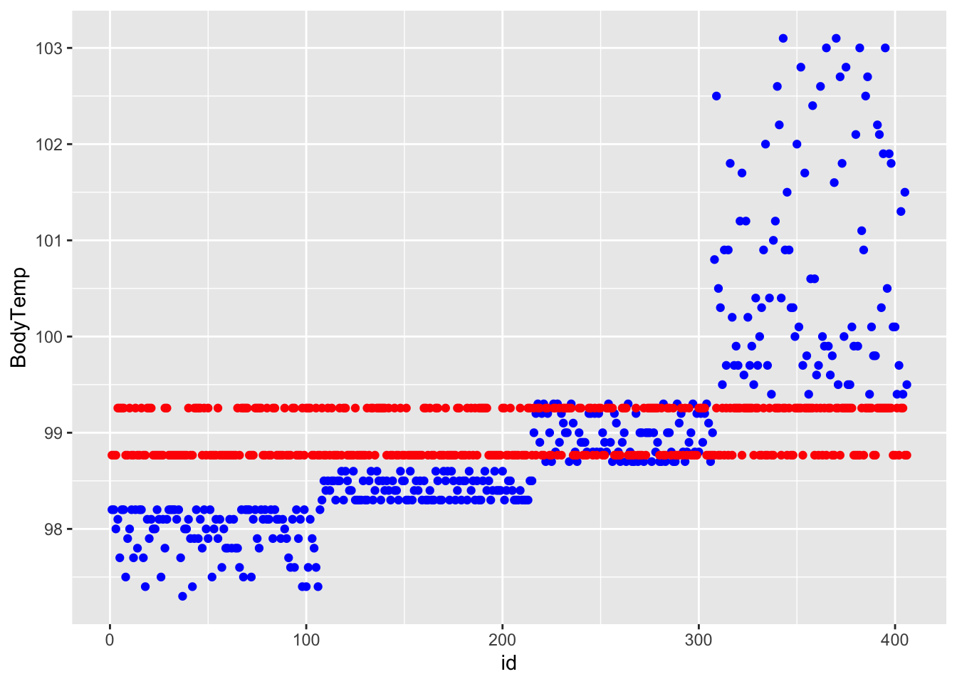
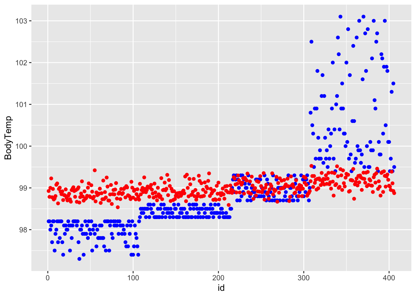
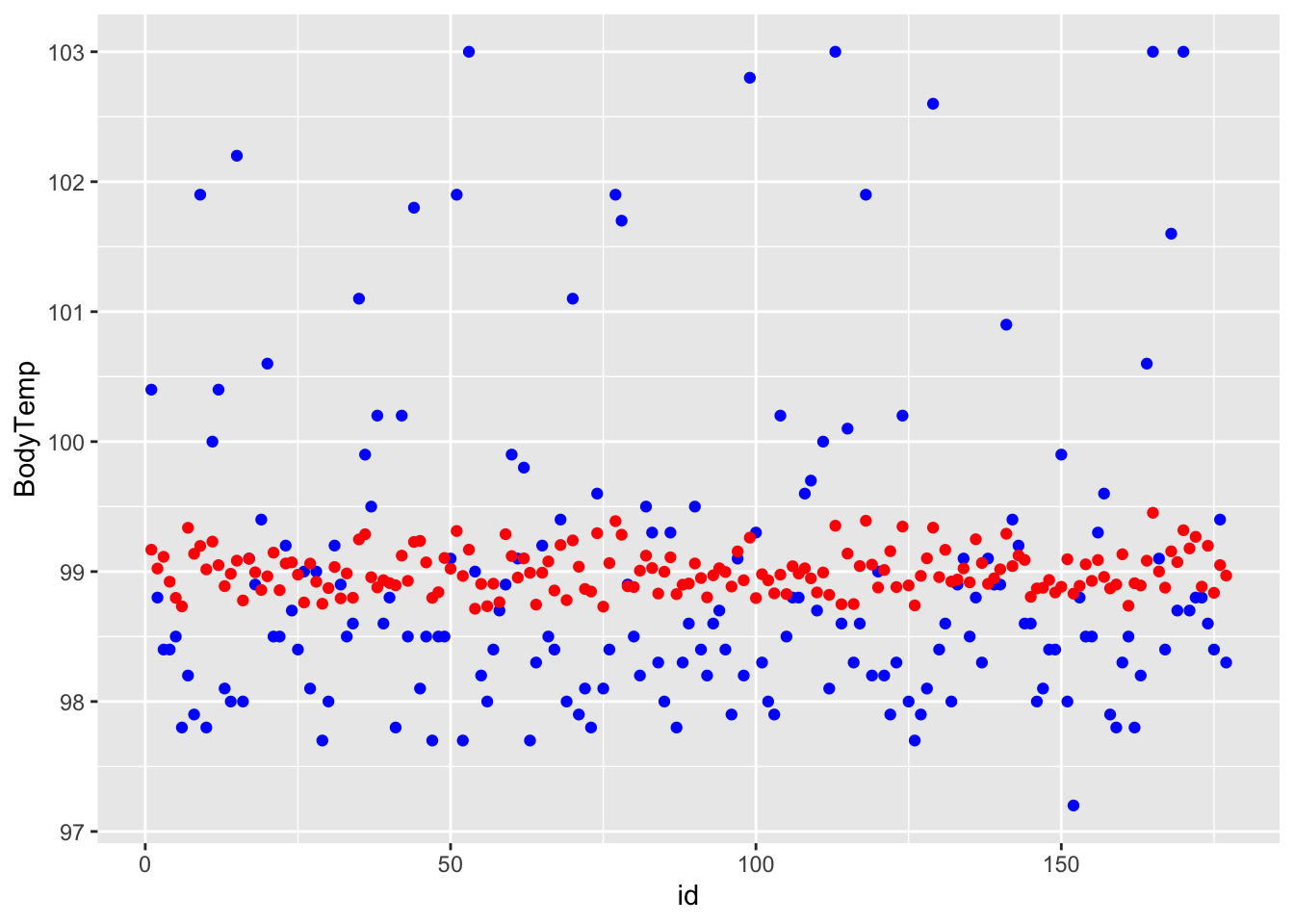
last_fit <- final_wf_rf %>% fit(test_data)
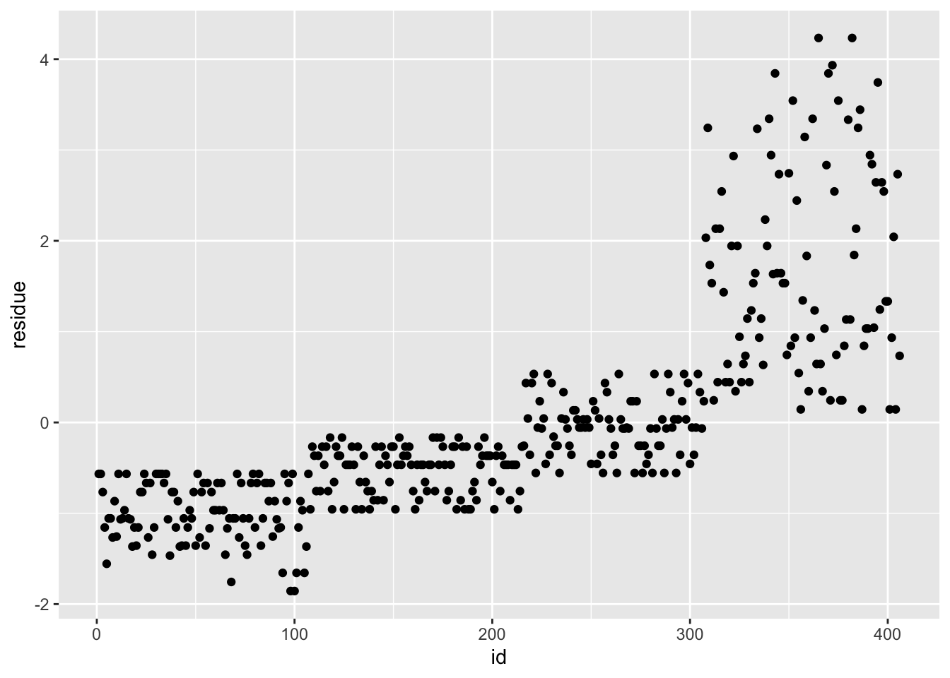
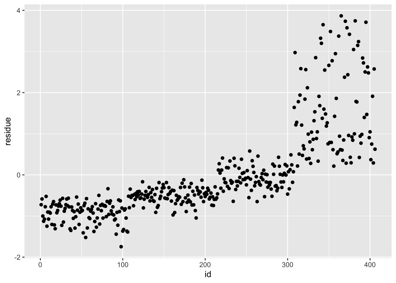
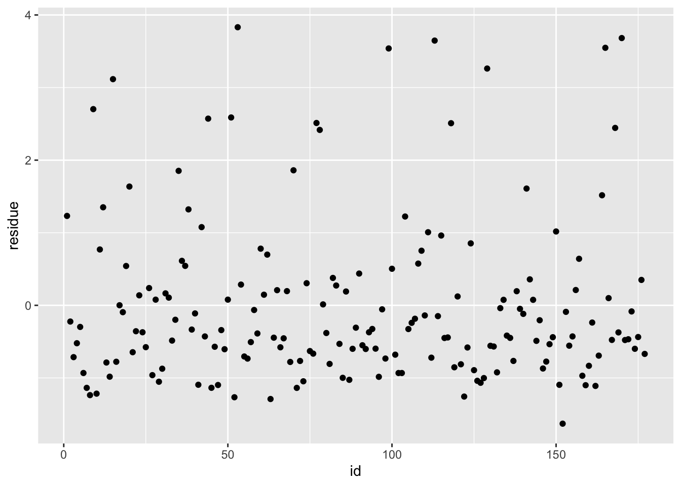
df_rf_last <- last_fit %>% augment(test_data) %>% select(.pred, BodyTemp) %>% mutate(residue = BodyTemp - .pred)
df_rf_last$id <- seq.int(nrow(df_rf_last))
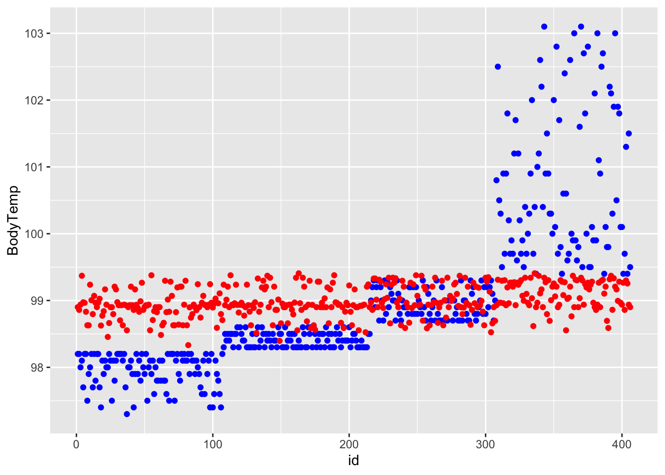
ggplot() + geom_point(data = df_rf_last, aes(x = id, y = BodyTemp), color = "blue") + geom_point(data = df_rf_last, aes(x = id, y = .pred), color = "red")
## # A tibble: 1 × 3
##   .metric .estimator .estimate
##   <chr>   <chr>          <dbl>
## 1 rmse    standard        1.12